ESE 471: Digital Communication Theory and Systems
Want to know more digital communication theory? Want to know how to design communication systems? While communication systems have become more and more ubiquitous, more efficient, and more advanced, engineers have designed new technologies using the same framework of tools: orthogonal signals; optimal Bayesian detection, and designing to ensure robustness to the channel. This course covers topics in each segment. This page provides resources for those wanting to learn more on their own, as well as information about how ESE 471 is taught at Washington University in St. Louis. These resources are provided by Dr. Neal Patwari, who created the videos and the course notes. If you use them, please cite these resources as:
Neal Patwari, ESE 471: Digital Communication Theory and Systems, Course Notes and Videos, April 2021, https://patwarilab.com/ese471.html.
Notes:
My ESE 471 course lecture notes for 2021 are freely available. These are divided by lecture number, and also by section headings. Multiple sections might be covered in one class session. The Lecture heading states what topics are covered, as well as the readings assigned to students for that class session.
Readings:
Our primary text is Michael Rice, Digital Communications: A Discrete-Time Approach, ISBN-13: 978-1790588565. This self-published paperback is available for $60.
Objectives and Topics:
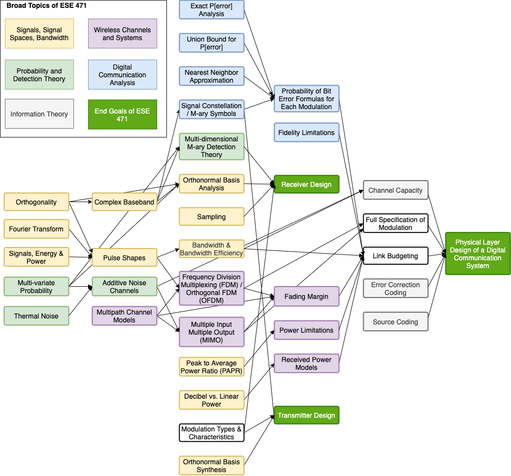 Primarily, the course objectives are to understand how digital communications transmitters and receivers send and receive data; to be able to build a Bayesian optimal detector and calculate its error probabilities for a particular modulation; and to design a communication system to meet specifications. There are multiple skills needed to get to these objectives, as outlined here as a flow diagram.
Homework Assignments:
There are ten homework assignments in the class, approximately once per week. For those lectures below which list a homework assignment, this is an assignment students can complete after completing the given lecture material. If none is listed for a lecture, this means that the material is covered in the following homework assignment. Please note that I do not make solutions publicly available for these asssignments.
Course by Class Session:
Class Session 1
The first lecture of my semester presents the syllabus and gives a big-picture look at the topics covered in the course, how they lead from one to another, to eventually get to the learning outcomes of the course. These outcomes are to be able to design a transmitter and receiver, and to use link budget analysis and information theoretic tools to design a communication system to meet the specifications given. No videos have yet been created for this first lecture.
Class Session 2
This lecture presents the most critical concepts needed to study how signals are used to send information in digital communication systems: power, energy, and orthogonality. The last property requires some motivation, so I describe how orthogonality can be seen as the receiver's ability to separate one signal from another. I do some examples of orthogonality.
Video Segments:
- Signals, Power, and Energy (7:10)
- Why Study Orthogonality? (5:33)
- Orthogonality Definition and Examples (9:09)
Homework:
Class Session 3
This lecture applies the concept of orthogonality to describe how a digital communication transmitter and receiver work. Specifically at the transmitter: how they use K orthogonal waveforms; how they send one of M possible linear combinations of those waveforms; and how that choice of one of the M conveys bits in a message. At the receiver, the fact that the waveforms are orthogonal to each other allows it to separate them and compute the amounts of each waveform sent, and thus guess which of the M possible linear combinations was sent, which indicates which bits were meant to be sent.
Video Segments:
Class Session 4
This lecture describes / reviews the frequency transforms we use in digital communication (and why); and the Fourier transform properties we use the most in the design of pulse shapes. Finally we cover sampling and aliasing, using these frequency domain techniques.
Video Segments:
Homework:
Class Session 5
In this lecture I introduce pulse amplitude modulation (PAM) and show what the signal looks like in the time domain at the transmitter. I then talk about the matched filter at the receiver and show that it can be looked at as a filter (a convolution) or as an integral of the signal multiplied by the waveform (correlation). Finally, to keep one symbol from contributing interference to subsequent symbols (inter-symbol interference), we can use the Nyquist Filtering Theorem to describe how to design a pulse shape, starting in the frequency domain. I describe this with a scissors and paper craft activity.
Video Segments:
Homework:
Class Session 6
This class session is used to show students how to use Matlab or Python to complete the projects they do over the semester. No videos have yet been created for this lecture.
Class Session 7
In this lecture, I introduce quadrature amplitude modulation (QAM), its basis functions and some example constellation diagrams, including for phase shift keying (PSK) and amplitude PSK (APSK). We then show how to calculate the average bit energy and average symbol energy. Finally, we introduce complex baseband notation as an equivalent way to represent the two orthogonal basis functions.
Video Segments:
Class Session 8
This lecture shows what a PAM and QAM digital communication signal looks like in the time domain, in particular when using a square root raised cosine (SRRC) pulse shape. Complex baseband notation is used. The property of 'envelope' is introduced, and offset-QPSK is introduced to show how a short time delay between in-phase and quadrature components can make the envelope relatively constant over time. Finally, we introduce two versions of M-ary FSK, coherent and non-coherent, and derive the frequency offset between carriers needed for each type of receiver.
Video Segments:
Homework:
Class Session 9
This lecture has two segments. First, I describe frequency division multiplexing (FDM), in particular orthogonal FDM (OFDM). OFDM uses a set of orthogonal waveforms in combination, and I explain how it is like a combination of QAM and M-ary FSK. I show how the transmitted signal can be computed using a Fast Fourier Transform (FFT). In the second segment, I introduce some of the probability tools that you need to be able to evaluate the probability of bit error of particular communications modulations. One pre-req of the course is an undergrad probability course, so I do an example to refresh your memory of how to use probability density functions and probability mass functions to compute probabilities.
Video Segments:
Class Session 10
This lecture covers Bayesian detection theory. First, we cover the Bayesian minimum probability of error goal, and use it to derive a general expression for the detection test (algorithm) to decide which out of two symbols were sent. The rule generally applies to when the noise is any distribution. We then get specific to the case when the distributions are Gaussian. I derive formulas for the general additive uncorrelated Gaussian noise case, and talk about the effect of different probabilities of two different symbols. Finally I provide the formula for the specific case in which the symbols are equally probable.
Video Segments:
Homework:
Class Session 11
This lecture is all about noise. In particular, thermal noise, which is added in to every receiving antenna. The videos explain, from information about the physics of thermal noise, how we can show that our symbols samples (after the matched filter) will contain additive, uncorrelated, and Gaussian noise. I explain also how to calculate the power (variance) of the noise that contributes to the received signal.
Class Session 12
This lecture derives the optimal decision rule for M-ary, K-dimensional constellations, showing that the rule is, for equally-probable symbols, to pick the symbol vector closest to the measured vector. Any single decision boundary for this rule is a line, the perpendicular bisector of the line segment between the two symbol vectors, which is proven in the 2nd video. In combination across all symbols, the decision regions become a Voronoi diagram.
Class Session 13
In this lecture, I derive the probability of symbol error formula for M-ary pulse amplitude modulation (PAM), and then show how to calculate an approximate probability of bit error from a probability of symbol error when we use Gray coding. Decibel notation is covered because we often refer to Eb/N0 in dB terms, and will use dB notation extensively in link budget analysis.
Video Segments:
Homework:
Class Session 14
In this lecture, I derive the union bound for the probability of symbol error, first in general, and then for a digital communication receiver. Then I present the nearest neighbor approximation. Finally I do an example of the two types of probability of symbol error formulas for M=8 Box QAM.
Video Segments:
Class Session 15
This lecture shows how to derive the probability of symbol and bit error in QAM / PSK communication systems in additive uncorrelated noise. Note that in the remaining videos I used vector ai instead of vector si to denote symbol vector i, and 'r = [r0, ... rK-1]' instead of 'x = [x0, ..., xK-1]' to denote the received vector.
Video Segments:
- 2x4 rectangular QAM Probability of Error Example (12:29)
- Binary FSK Coherent Receiver (5:30)
- Binary FSK: Noncoherent Receiver (9:02)
- Differential BPSK (12:29)
Homework:
Class Session 16
This lecture presents the probability of bit and symbol error in M-ary FSK (for both coherent and non-coherent reception); and then compares the many modulations we've considered so far in terms of probability of bit error vs. Eb/N0, bandwidth, and bandwidth efficiency.
Video Segments:
- M-ary Noncoherent FSK Probability of Error (14:06)
- M-ary Coherent FSK Probability of Error (v2) (5:27)
- Modulation Comparison (10:31)
- Bandwidth Efficiency (9:14)
Class Session 17
This lecture covers link budgets and received power (path loss) models. Generally speaking, the purpose of this material is to be able to analyze the design of a wireless communication system, relating parameters like transmit power, range, probability of bit error, and bandwidth.
Video Segments:
- Wireless System Design Relationships (4:06)
- Received Power Models (15:59)
- Calculation of EbN0 (4:03)
- System Design Example: Peer to Peer Microwave Link (14:59)
Homework:
Class Session 18
This lecture covers link budgets, in particular how to design a wireless link to achieve constraints on probability of bit error, bandwidth, bit rate, transmit power, and other parameters. Sometimes we don't know whether designing from the probability of bit error constraint will result in a bandwidth that is too high, or vice versa. So we sometimes have to solve from both directions in order to achieve both constraints. I show the spreadsheet I use for link budget calculations.
Video Segments:
Class Session 19
This lecture is on source coding: How we use entropy and entropy rate to quantify the number of bits of information in a random variable or random source (sequence of samples, for example). The source coding theorem tells us that if we try to encode our source with rate less than the entropy rate, we'll see a significant error rate.
Video Segments:
- Intro to Entropy with Examples (14:58)
- Joint Entropy and Entropy Rate (13:39)
- Shannon Source Coding Theorem (5:10)
Homework:
Class Session 20
This lecture covers Shannon's Channel Capacity theorem and forward error correction coding. The capacity bound, and the difference in bandwidth efficiency between most of our modulation methods and the bound, motivate using error correction. Systematic linear block codes are covered as an example of a forward error correction method.
Video Segments:
Class Session 21
This lecture covers how multipath fading causes the signal to be low in amplitude some of the time as a result of the fat that the antenna adds a random complex value for each multipath component. One way to be robust is to put in a lot of leeway in your link budget. Other ways involve using multiple antennas at the receiver, at the transmitter, or at both TX and RX. The latter video covers examples of these three methods.
Video Segments:
Homework:
Comments or Corrections
Please contact Neal Patwari with questions, comments, or corrections.